Solving an ODE that has a convolution with RK4
In this note I document stuff I remembered doing back when I was taking Numerical Methods I.
We’ll get the idea from Euler method, then extend it up to a family of method called Runge-Kutta. The Runge-Kutta 4th order is the final step, and is considered the one ring to rule all ODEs.
Euler method
Let say we have a first-order differential equation problem
\[\begin{align} \dfrac{dx}{dt} - f(t, x) = 0,\ x(t_0) = x_0 \end{align}\]
This means that we know where we were initially: $x$ at $t_0$. Now, we move forward to $t_1$, meaning we move a distance of $\Delta t = t_1-t_0$. Provided that we also know how $x$ changes with respect to $t$–that’s $dx/dt=f(t, x)$, we can approximate $x$ at $t_1$ as (using Taylor expansion)
\[ x(t_1) := x(t_0+\Delta t) = x(t_0) + \Delta t f(t_0, x_0) \]
Since we know where we were ($x(t_0)=x_0$), and we definitely know how to calculate $f(t_0, x_0)$, we can calculate $x_1$. Iteratively, this is
\[ x_{n+1} = x_n + \Delta t f(t_n, x_n) \]
For small enough $\Delta t$, the numerical solution should not deviate much from the exact solution. Of course, this is a very simple kind of thing. The error order is quite large, $O(\Delta t^2)$.
Modified Euler method
To improve the Euler method, we add to our toolkit something called predictor-corrector. This p-d thing is based on the idea of averaging the value of $f(x,t)$ at the beginning and end of each time we move forward. Mathematically speaking,
\[ x_{n+1} = x_n + \dfrac{1}{2}\Delta t(f(t_n, x_n)+ f(t_n+\Delta t, x_{n+1})) \]
The glaring problem lies at the term $f(t_n+\Delta t, x_{n+1})$. We’re supposed to calculating $x_{n+1}$, now we have to use what we’re finding to calculate itself? Well, how about approximate it? How to approximate it, you might ask? Simply use the Euler method.
\[ x^P_{n+1} = x_n + \Delta t f(t_n, x_n) \]
We will not take this as the final answer. We use it as a predictor. Now that we’ve obtained $x_{n+1}$, stuff it into the original equation
\[ x_{n+1} = x_n + \dfrac{1}{2}\Delta t(f(t_n, x_n)+ f(t_n+\Delta t, x^P_{n+1})) \]
Now let us actually write a code. We’ll use Python here. Say we have a first-order differential equation problem.
\[ \dfrac{dx}{dt} = \cos(\omega t)+x, x_0 = 1.0 \]
Here’s the code that works,
import numpy as np
import matplotlib.pyplot as plt

omega = 1.0

def f(t, x):
    return np.cos(omega*t) + x

time_step = 0.001
tmax = 10
t_range = np.arange(0, tmax, time_step)
x_num = np.zeros([len(t_range)])
x_num[0] = 1.0 # initial condition


def heun(f, t_range, time_step):
    '''
    Modified Euler method, also known as heun method (is this guy a Korean?)
    '''

    for j in range(len(t_range)-1):
        t_n = t_range[j]
        x_n = x_num[j]
        h1 = time_step * f(t_n, x_n)
        x_p = x_n + h1
        h2 = time_step * f(t_range[j+1], x_p)
        x_num[j+1] = x_num[j] + 0.5*(h1+h2)

    return x_num

x_num = heun(f, t_range, time_step)

plt.plot(t_range, x_num)
The modified Euler method is one of a family of methods called second-order Runge-Kutta methods.
Runge-Kutta method
In deriving the modified Euler formula, we’ve made the predictor by evaluating $f(t_{n+1}, x_{n+1})$ at $t_{n+1}=t_n + \Delta t$ and $x_{n+1} = x_n + h_1$. A straightforward generalization would be twisting the predictor (now let us replace $h$ by $r$)
\[\begin{align} r_1 = \Delta t f(t_n, x_n),\newline r_2 = \Delta t f(t_n+\alpha\Delta t, x_n + \beta r_1),\newline x_{n+1} = x_n + a r_1 + b r_2 \end{align}\]
Upon replacing $a=b=1/2$ and $\alpha=\beta=1$, we obtain the modified Euler version. Now, we cannot choose $a, b, \alpha, \beta$ arbitrarily. In fact, there’s some constraints on them, namely
\[ a+b = 1,\ \alpha b = 1/2,\ \beta b = 1/2 \]
These constraints originate from the uniformity of the Taylor expansions of $x_{n+1}$ in two different ways whose detailed calculation is beyond the scope of this note.
Higher-order Runge-Kutta methods are obtained when we further generalize the $x_{n+1}$ formula by adding more predictors. In essence, what’s really going on after each update of predictor is the corrector becoming more and more accurate.
Fourth-order Runge-Kutta
Here I list the formula for the fourth-order Runge-Kutta method, also physicists’ favourite one.
\[\begin{align} r_1 = \Delta t f(t_n, x_n),\newline r_2 = \Delta t f(t_n + \dfrac{1}{2}\Delta t, x_n + \dfrac{1}{2}r_1),\newline r_3 = \Delta t f(t_n + \dfrac{1}{2}\Delta t, x_n+\dfrac{1}{2}r_2),\newline r_4 = \Delta t f(t_n+\Delta t, x_n+r_3),\newline x_{n+1} = x_n + \dfrac{1}{6}(r_1+2r_2+2r_3+r_4) \end{align}\]
And the Python implementation.
def rk4(f, t_range, dt):
    '''
    Runge-Kutta fourth-order. Kutta means `dog` in Hindi somehow (with bad meaning).
    '''

    for j in range(len(t_range)-1):
        t_n = t_range[j]
        x_n = x_num[j]
        r1 = dt * f(t_n, x_n)
        xp1 = x_n + 0.5*r1
        r2 = dt * f(t_n+0.5*dt, xp1)
        xp2 = x_n + 0.5*r2
        r3 = dt * f(t_n+0.5*dt, xp2)
        xp3 = x_n + r3
        r4 = dt * f(t_n+dt, xp3)
        x_num[j+1] = x_num[j] + 1/6*(r1+2*r2+2*r3+r4)

    return x_num
Higher-order ODEs
We can actually solve for higher order ODEs. Consider the second-order ODE given by
\[ \ddot{x} - f(t, x, \dot{x})=0, \]
where $f$ is a function of $t, x, \dot{x}$. This second-order ODE can be rewritten as a system of two first-order ODEs by introducing one more variable, $u=dx/dt$.
\[\begin{align} \dot{x} = u,\newline \dot{u} = f(t, x, u) \end{align}\]
Then, each first-order coupled ODE above can be solved simultaneously with RK4 method.
Case in point: damped harmonic oscillator
The damped harmonic oscillator’s equation of motion reads,
\[ \begin{align} \ddot{x}(t) + \Omega_0^2 x(t) + \int_0^t \dot{\kappa}(t-\tau)x(\tau)d\tau = 0\newline \ddot{x}(t) = -\left[\Omega_0^2 x(t)-\int_0^t \dot{\kappa}(t-\tau)x(\tau)d\tau\right]. \end{align} \]
The EoM above can be rewritten into two coupled first-order ODE,
\[ \begin{align} \dot{x} = f(v) = v,\newline \dot{v} = g(t, x) = -\left[\Omega_0^2 x-\int_0^t \dot{\kappa}(t-\tau)x(\tau)d\tau\right] \end{align} \]
In this case, the generalized RK4 method would be
\[ \begin{align} r_1 = \Delta t f(v_n),\quad k_1 = \Delta t g(t_n, x_n),\newline r_2 = \Delta t f(v_n + \dfrac{1}{2}k_1),\quad k_2 = \Delta t g(t_n+\dfrac{1}{2}\Delta t, x_n + \dfrac{1}{2}r_1),\newline r_3 = \Delta t f(v_n + \dfrac{1}{2}k_2),\quad k_3 = \Delta t g(t_n+\dfrac{1}{2}\Delta t, x_n+ \dfrac{1}{2}r_2),\newline r_4 = \Delta t f(v_n+k_3),\quad k_4 = \Delta t g(t_n+\Delta t, x_n+r_3),\newline v_{n+1} = v_n + \dfrac{1}{6}(k_1+2k_2+2k_3+k_4),\newline x_{n+1} = x_n + \dfrac{1}{6}(r_1+2r_2+2r_3+r_4). \end{align} \]
Now let us actually implement this scheme using Python. The hardest part is probably the convolution integral. Let us now consider a naive version of doing this. The integral in discrete sense,
\[ \begin{align} \int_0^t \dot{\kappa}(t-\tau)x(\tau)d\tau = \sum_{j=0}^{k-1} \dot{\kappa}((k-j)\Delta t)x(j\Delta t)\Delta t \end{align} \]
This can be naively implemented in Python by
convo = 0
if n == 0:
    return -Omega**2*x_n
else:
    for j in range(n):
        convo += kappad_vals[n-j]*x_num[j]*dt
where kappad_vals and x_num are the two signals being convoluted. It’s time to incorperate this into our RK4 scheme
def kappa_dot(gamma, omega_c, t):
    return -(gamma*omega_c**3*t)/(1+(omega_c*t)**2)**2

def f(v):
    return v

def g(Omega_0, kappad_vals, x_num, dt, n, x_n):
    '''
    k will dictate time, i.e. t_n = t_range[n]
    '''
    convo = 0
    if n == 0:
        return -Omega_0**2*x_n
    else:
        for j in range(n):
            convo += kappad_vals[n-j]*x_num[j]*dt

    return -Omega_0**2*x_n - convo

def simDQHO_RK4(tmax, dt, Omega_0, omega_c, gamma):
    '''
    Four free parameters
    '''
    t_range = np.arange(0, tmax, dt)

    kappad_vals = [kappa_dot(gamma, omega_c, t) for t in t_range]

    x_num = np.zeros([len(t_range)])
    v_num = np.zeros([len(t_range)])
    v_num[0] = 0 # initial condition (no initial velocity)
    x_num[0] = 1.0 # initial condition

    for n in range(len(t_range)-1):
        t_n = t_range[n]
        x_n = x_num[n]
        v_n = v_num[n]

        r1 = dt * f(v_n)
        k1 = dt * g(Omega_0, kappad_vals, x_num, dt, n, x_n)
        xp1 = x_n + 0.5*r1
        vp1 = v_n + 0.5*k1

        r2 = dt * f(vp1)
        k2 = dt * g(Omega_0, kappad_vals, x_num, dt, n, xp1)
        xp2 = x_n + 0.5*r2
        vp2 = v_n + 0.5*k2

        r3 = dt * f(vp2)
        k3 = dt * g(Omega_0, kappad_vals, x_num, dt, n, xp2)
        xp3 = x_n + r3
        vp3 = v_n + k3

        r4 = dt * f(vp3)
        k4 = dt * g(Omega_0, kappad_vals, x_num, dt, n, xp3)

        x_num[n+1] = x_n + (1/6)*(r1+2*r2+2*r3+r4)
        v_num[n+1] = v_n + (1/6)*(k1+2*k2+2*k3+k4)

    return t_range, x_num
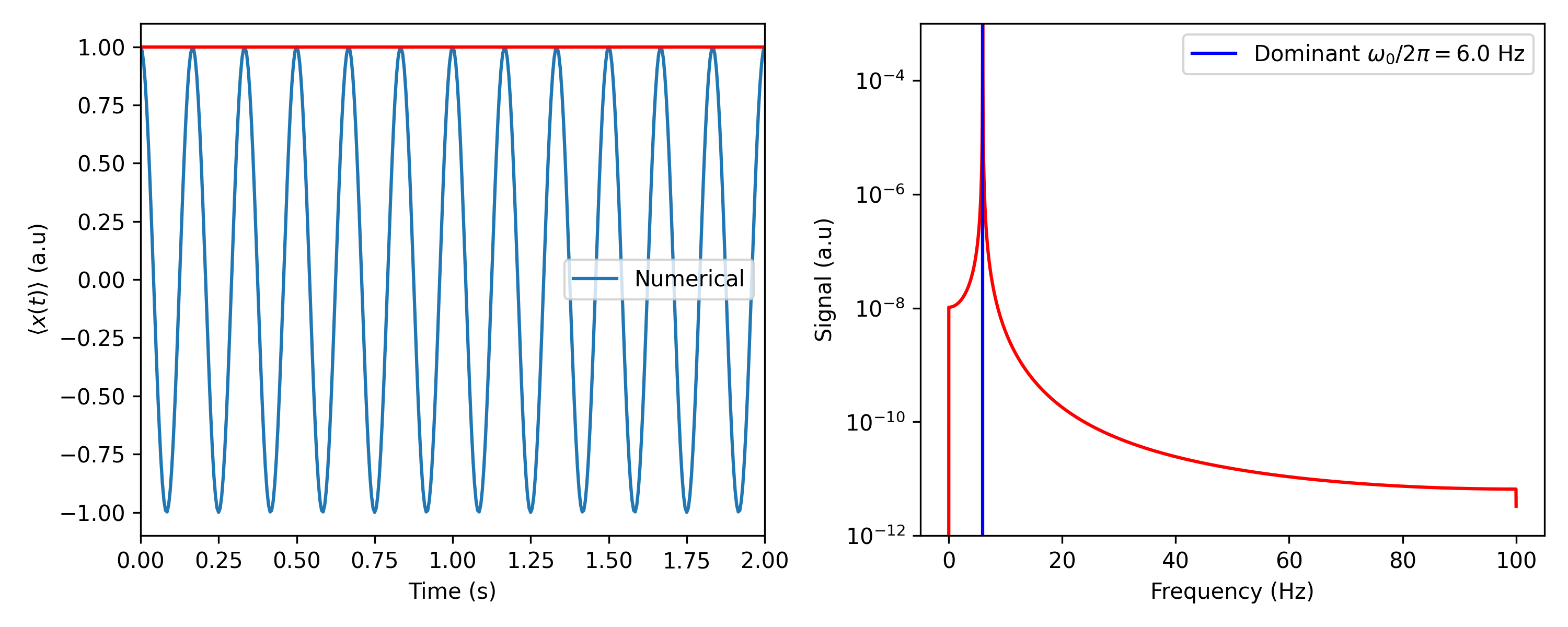
Let us now demonstrate the case when the frequency cut-off being 0. In such case, there should be no damping effect. The Fourier transform of the signal should have a dirac-delta-like peak at the frequency $\Omega_0$, chosen to be $6$ Hz in this case.
dt = 0.5e-2
tmax = 50
Omega_0 = 2*np.pi*6
omega_c = 0*Omega_0
gamma = 1

t_range, x_num = simDQHO_RK4(tmax, dt, Omega_0, omega_c, gamma)

fs = 1/dt #sampling rate
(freq, S) = scipy.signal.periodogram(x_num, fs, scaling='density')
dominant_freq = freq[np.argmax(S)]

fig, axes = plt.subplots(nrows=1, ncols=2, figsize=(10, 4))
axes[0].plot(t_range, x_num, label='Numerical')
axes[0].set_xlabel('Time (s)')
axes[0].set_ylabel(r'$\langle x(t)\rangle$ (a.u)')
axes[0].set_xlim([0, 2])
axes[0].axhline(1.0, color='red')
# axes[0].axvline(1/6, color='green')
axes[0].legend()
axes[1].semilogy(freq, S, color='red')
axes[1].axis(ymin=1e-12, ymax=1e-3)
axes[1].set_xlabel('Frequency (Hz)')
axes[1].set_ylabel('Signal (a.u)')
axes[1].axvline(dominant_freq, color='blue', label='Dominant $\omega_0/2\pi=$'+f'{np.round(dominant_freq,3)}'+' Hz')
axes[1].legend()
fig.tight_layout()
fig.savefig('./figures/DQHO_no_coupling.png', dpi=300)
Indeed, the oscillator completes one period of oscillation in $1/6$ second.

Oscillation of an undamped harmonic oscillator.
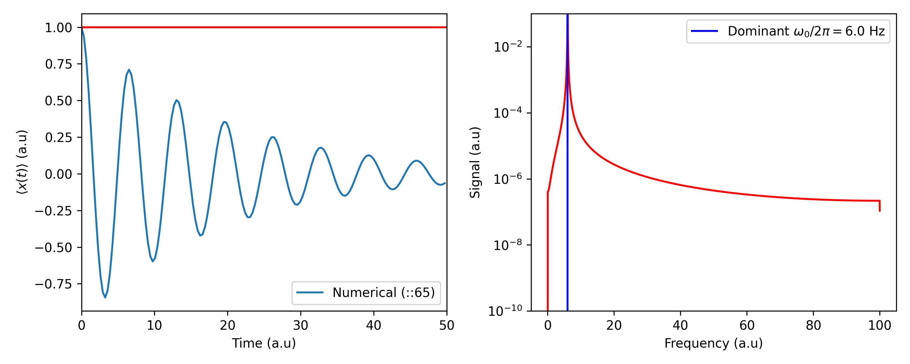
We now consider a cut-off frequency of 50% of the oscillator. The Fourier transform of the signal is now no longer a dirac-delta-like function. Notice how other frequency components other than the dominant frequency is enhanced. This is expected, since
\[ \dfrac{1}{2\pi}\int_{-\infty}^{\infty} e^{-\gamma t}e^{-i\omega_0 t}e^{-i\omega t}d\omega \]
has the form of a Lorentzian function.

Oscillation of a damped harmonic oscillator $(\omega_c=0.5\Omega_0)$.
A question is left for readers.
Can we see the overdamped effect?